Automated GC-MS Chromatogram Analysis: From Raw Signal to Quantified Peaks

Valentin Caries

Sep 12, 2026

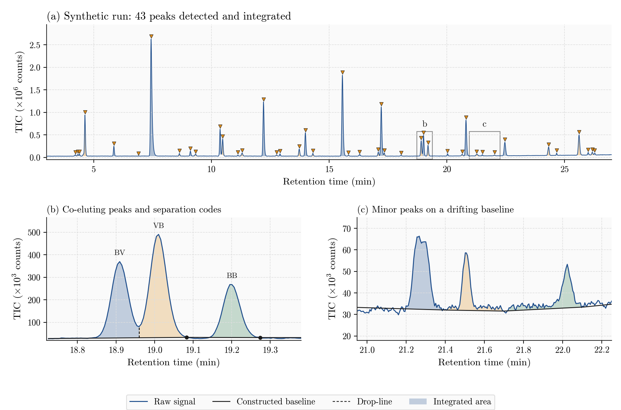
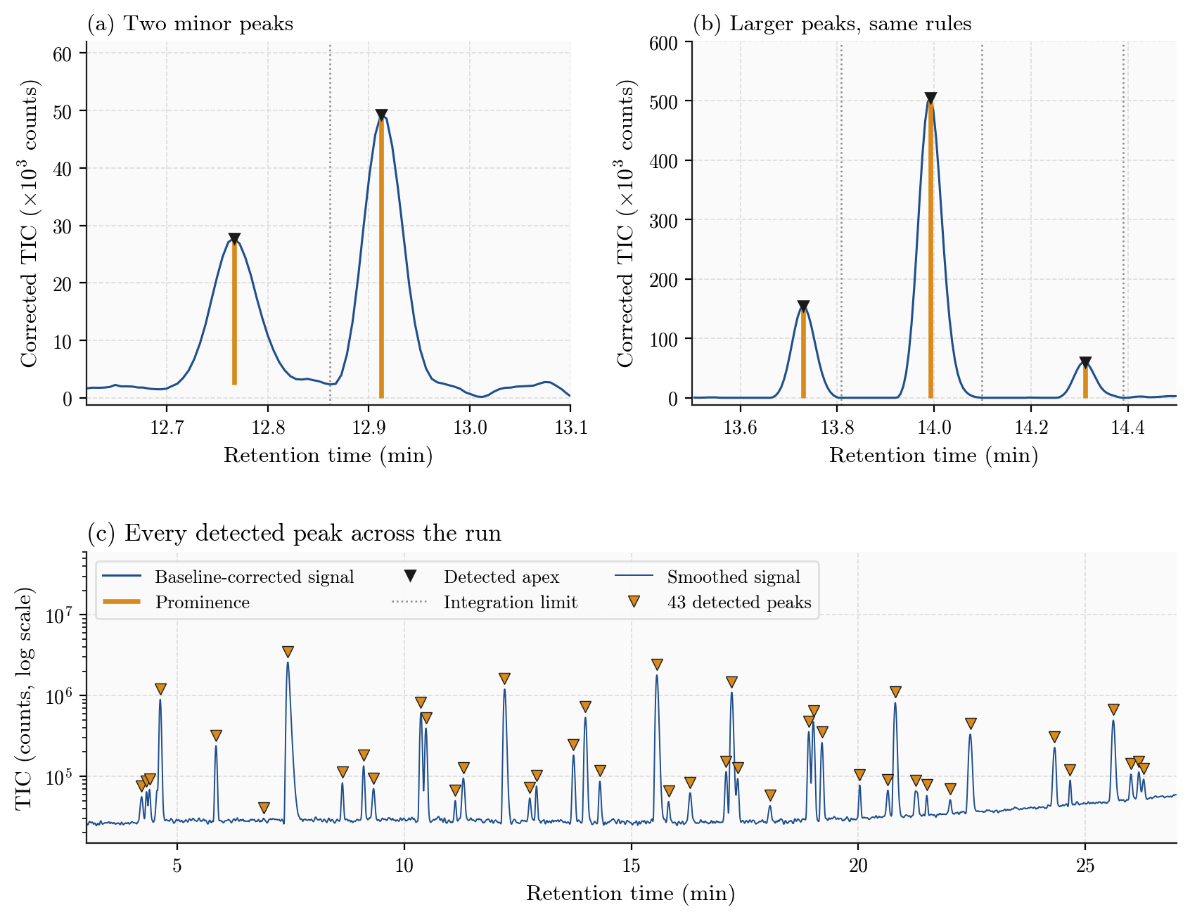
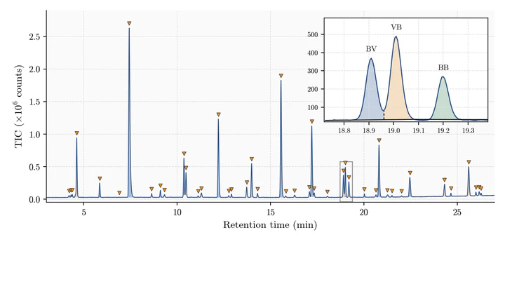A synthetic chromatogram processed end to end: every detected peak integrated, with a co-eluting triplet magnified

In one minute

I developed a Python package that automates the analysis of GC-MS chromatograms, from the raw instrument file to a table of quantified peaks. Gas chromatography coupled with mass spectrometry separates the compounds in a sample and records how much signal elutes at each instant. Each compound appears as a peak, and the peak’s area measures how much of it the sample contains. In practice, those peaks are often located, bounded and integrated by hand in vendor software, then copied into spreadsheets. The result depends on the operator, is slow to produce for many runs, and is hard to reproduce or audit afterwards.

The pipeline replaces that manual chain with a deterministic sequence of well-established signal-processing steps. It reads the vendor’s binary files directly and reconstructs the total-ion chromatogram. It smooths it with a Savitzky–Golay filter and estimates the baseline by asymmetric least squares. It then detects peaks by topographic prominence against a robust noise estimate and bounds each one at the valleys. Areas are measured by default with a reimplementation of the Agilent ChemStation integration methodology: a constructed baseline, drop-lines or valley baselines for merged peaks, and a peak separation code. Every stage is a pure function of its input and of one versioned parameter set, so the same run always yields the same numbers.

What this enables is a reproducible analysis that can be scripted over whole batches of runs, inspected peak by peak, and checked against manual results. The same library drives a command-line tool, a desktop application, self-contained interactive HTML reports in which any peak can be re-integrated with the mouse, and tidy CSV, JSON, Parquet or xlsx tables ready for statistical analysis.

About the figures. The data analysed by this project are confidential. Every chromatogram, figure and screenshot on this page was produced from synthetic data generated specifically for this demonstration. None of them corresponds to the real chromatograms processed by the software. The synthetic signal is nonetheless run through the package’s actual code, so what the figures show is what the software does.

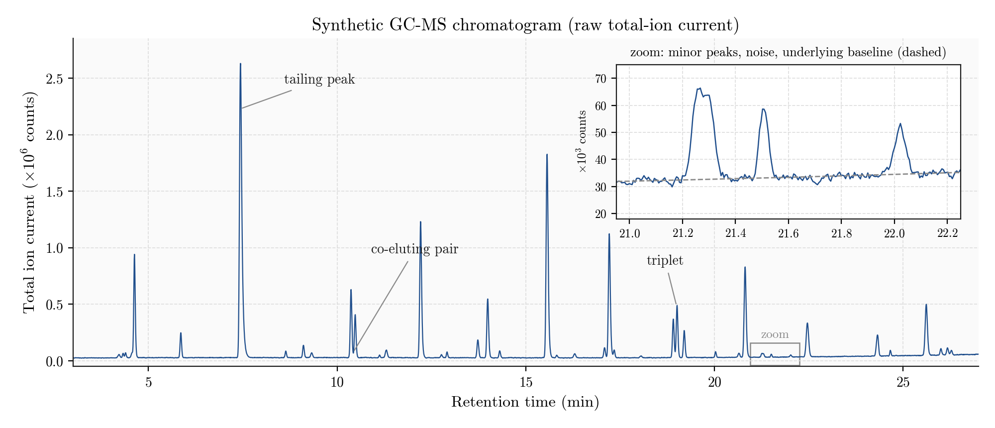
A synthetic chromatogram with every detected peak integrated, and two magnified regions — **Figure 1.** A synthetic run processed end to end. (a) The raw total-ion current, with each detected apex marked and each integrated area shaded. (b) Three co-eluting peaks: the first two share a baseline and are separated by a vertical drop-line, while the third returns to the baseline. The two-letter labels are the separation codes the integrator assigns. (c) Minor peaks on a slowly drifting baseline, each integrated above its own constructed baseline. *(Click any figure to open it full size.)*

Highlights

An end-to-end pipeline. Binary parsing, smoothing, baseline correction, noise estimation, detection, integration, identification by retention time, relative quantification and validation, with the algorithms selected by configuration behind interchangeable interfaces.
A vendor methodology, reimplemented from its documentation. Peak clusters, peak-valley-ratio arbitration between drop-lines and valley baselines, baseline penetration handling, height, width and separation codes. Areas are reported in explicitly labelled units.
Validated against manual work. Detection recovers 93 % of the manually identified compounds within 3 s (median retention-time error ≈ 0.1 s). Given the operator’s own integration limits, areas agree with manually integrated reference areas to a median of 3.5 % on baseline-resolved peaks.
Reproducible by construction. A frozen, hashable parameter set, a provenance trail on every signal, and a golden-file regression test that freezes every detected apex and boundary.
Usable by non-programmers. A command-line interface, a desktop GUI shipped as a standalone Windows executable, and interactive reports that need nothing but a browser.

Why automate chromatogram analysis?

A GC-MS run produces thousands of scans, and a rich sample can contain well over a hundred distinguishable peaks. Turning that into numbers usually involves three manual steps: recognising which peaks matter, deciding where each one starts and ends, and integrating it. Each step hides a judgement call. Where exactly is the baseline under a peak sitting on a drifting background? Where do two overlapping peaks separate? Is a small bump a compound or noise?

When those decisions are made by eye, three problems follow. Reproducibility: two operators, or the same operator a month later, will not draw identical limits, and the area moves with the limits. Traceability: a number in a spreadsheet does not record how it was obtained. Scale: the effort grows linearly with the number of runs, which quickly becomes the bottleneck of a study.

The goal of this project was therefore not only to compute areas, but to make every decision explicit, parameterised and repeatable, and to prove on real data that the automated result reproduces the manual one before relying on it.

From raw file to signal

The instrument writes each acquisition as a binary file in a legacy vendor format. Rather than depend on proprietary software or a native toolkit, the package includes a dependency-free parser written with the standard library and NumPy. It reads the file header (sample name, method, acquisition time) and the scan directory, which stores the retention time and the total ion current of every scan. The total-ion chromatogram (TIC), the sum of all ion intensities in each scan, can therefore be reconstructed losslessly without decoding the individual mass spectra. The binary layout is documented in the parser itself, so the format specification lives next to the code that implements it.

A raw synthetic chromatogram with a zoom on minor peaks and baseline noise — **Figure 2.** The synthetic raw signal used throughout this page. Peaks span more than two orders of magnitude, some tail, some co-elute, and the baseline rises slowly towards the end of the run. The zoom shows what is invisible at full scale: minor peaks, correlated scan-to-scan noise, and the underlying baseline the synthetic signal was built on (dashed).

The processing pipeline

Each stage is a pure function (input, parameters) → output, and every transformation of the signal appends its name to the signal’s provenance, so any output can be traced back to the exact processing that produced it.

flowchart TD A["Raw vendor file"] --> B["Parse
total-ion chromatogram"] B --> C["Smooth
Savitzky–Golay"] C --> D["Baseline
asymmetric least squares"] D --> E["Detect
prominence vs. noise"] E --> F["Bound
valley limits"] F --> G["Integrate
vendor method on the raw signal"] R["Reference table
(compound, retention time)"] --> H G --> H["Identify
retention-time matching"] H --> I["Quantify, validate, report"]

Smoothing

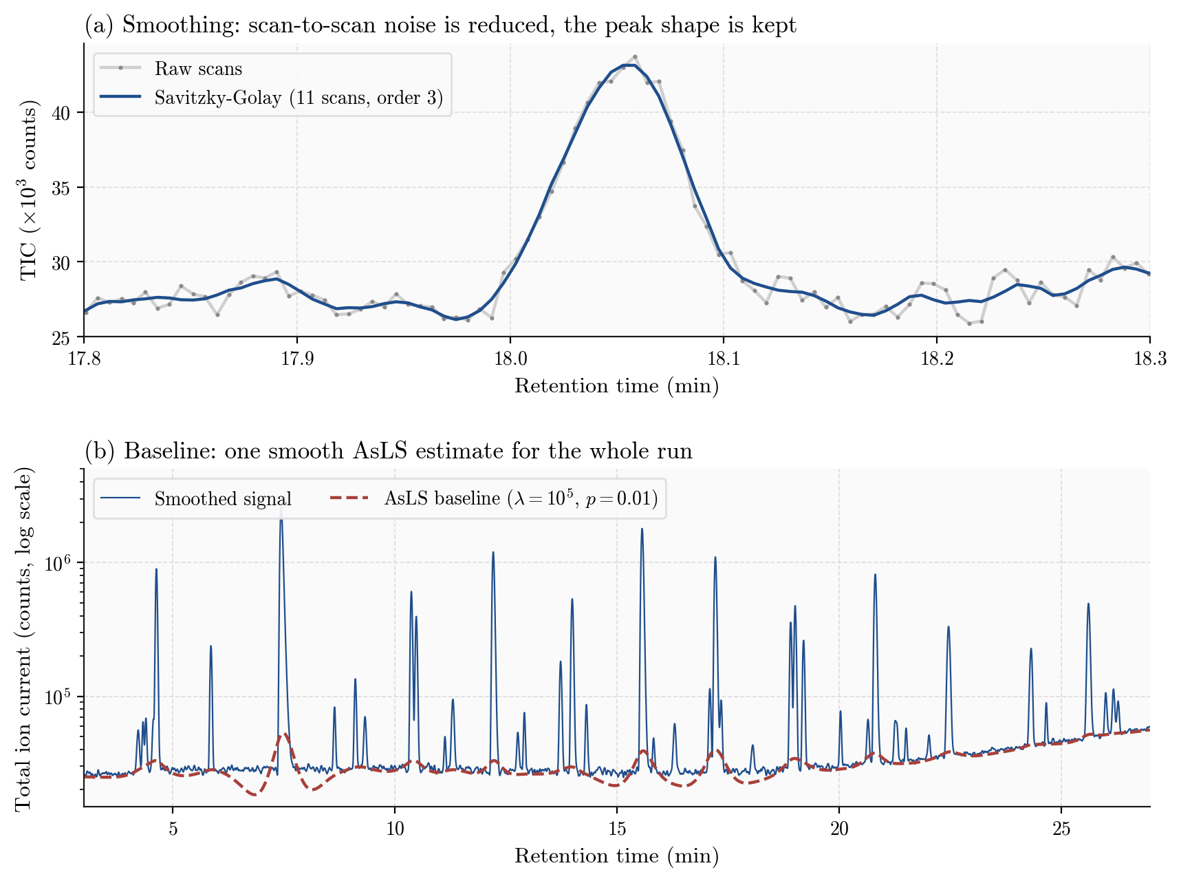
The TIC is first smoothed with a Savitzky–Golay filter: in a sliding window of 11 scans, a cubic polynomial is fitted by least squares and evaluated at the centre. Unlike a moving average, the local polynomial follows the curvature of a peak, so noise is reduced without flattening the apex or broadening the peak. That matters because detection and integration both depend on peak shape.

Baseline correction

A slowly varying background (column bleed, detector drift) is estimated by asymmetric least squares (AsLS). The baseline $z$ minimises a weighted fit to the signal $y$ plus a roughness penalty:

$$S = \sum_i w_i\,(y_i - z_i)^2 + \lambda \sum_i \left(\Delta^2 z_i\right)^2$$

The asymmetry is in the weights. Points above the current estimate, which are likely peaks, receive a small weight $p$, and points below receive $1 - p$. The fit is iterated so that the curve settles into the valleys and ignores the peaks. With the defaults $\lambda = 10^5$ and $p = 0.01$, each iteration solves a sparse linear system, which keeps the method fast on runs of several thousand scans. AsLS needs no manual anchor points and no assumed baseline shape.

Savitzky-Golay smoothing on a minor peak, and the AsLS baseline over the whole run — **Figure 3.** (a) Savitzky–Golay smoothing on a minor peak: the scan-to-scan noise is reduced while the peak keeps its height and width. (b) The AsLS baseline over the whole synthetic run, on a logarithmic scale. It follows the rising background, but it also bends under the largest peaks, where a single stiff curve cannot hug the valleys exactly. This is a known limitation of a single whole-run baseline. The corrected signal drives detection, while the default area measurement builds its own baseline locally from the peak limits (Figure 5).

Noise estimation and peak detection

Detection needs a sense of scale, so the noise level is estimated robustly from the median absolute deviation of successive differences:

$$\hat\sigma = \frac{\operatorname{median}\left(|\Delta y|\right)}{\sqrt{2}\times 0.6745}$$

Differencing removes the slow background, the median ignores the minority of large values that peaks contribute, and the two constants rescale the result to a Gaussian standard deviation.

Peaks are then the local maxima of the baseline-corrected signal whose topographic prominence exceeds a threshold: by default five times $\hat\sigma$, or an explicit minimum set by the analyst. Prominence measures how far a maximum rises above the higher of the two lowest points separating it from taller terrain on either side. Unlike raw height, it is insensitive to a residual offset and to a peak sitting on the flank of a larger one.

Integration limits

Each detected peak then receives two integration limits. Adjacent peaks are split at the valley, the minimum of the signal between their apexes, so windows meet without overlapping. This is the classical perpendicular-drop rule of chromatography data systems. The outermost edges descend from the apex to the first local minimum. An earlier boundary rule let windows overlap, so the same stretch of signal could be counted in two peaks. On the project’s data about 29 % of the total area was counted twice, and the valley rule removes that double counting without moving a single apex.

Measuring peak areas

Two families of integration methods

Integration is deliberately separated from detection. Detection produces geometry (an apex and two limits), while integration consumes limits and a signal. The seam is an explicit IntegrationBounds object that records where its limits came from: the detector, an operator who dragged them in the report, or an external result set. All three paths reach the same integrator, so a method can be compared with a reference without detection differences contaminating the comparison.

Methods are registered by name in a small registry, together with the signal each one requires. That detail prevents a quiet class of errors: numerical integration expects a baseline-corrected trace, while the vendor method builds its own baseline and would subtract one twice if handed the corrected signal. The registry therefore selects the right trace, and callers never have to know. Two numerical rules (trapezoidal and Simpson) integrate the AsLS-corrected signal. The default method follows the vendor methodology on the raw signal.

The vendor methodology: clusters, drop-lines and valley baselines

The default chemstation method implements the peak area measurement described in Agilent’s ChemStation documentation. Its detection algorithm was not in scope, only its area measurement, which it rebuilds in three steps.

Clustering. Peaks whose signal returns to the baseline between them are integrated independently. Adjacent peaks whose shared valley stays above the chord joining their outer limits form a cluster and share one baseline.
Drop-line or valley baseline. Inside a cluster, each valley is arbitrated by the peak-valley ratio defined below. Under a configurable threshold (10 by default), a vertical drop-line separates the two peaks. At or above it, the valley becomes an anchor of the baseline.
Area. The signal is integrated above the resulting piecewise-linear baseline, between each peak’s limits. Where the signal dips below the baseline, the negative contribution is clipped and the peak is flagged, so a baseline penetration can never subtract area.

The peak-valley ratio compares the smaller of the two neighbouring peak heights with the height of the valley between them, all measured above the provisional baseline:

$$\text{ratio} = \frac{\min(H_1, H_2)}{H_v}$$

A valley that comes down close to the baseline gives a large ratio and anchors it, while a shallow dip between merged peaks gives a small ratio and is cut by a drop-line.

Each peak also receives a height (its largest excursion above the baseline), a width following the vendor’s convention $\text{width} = \text{area}/\text{height}$, and a two-character separation code describing its start and end: B on the baseline, V at a drop-line, P where the baseline was penetrated.

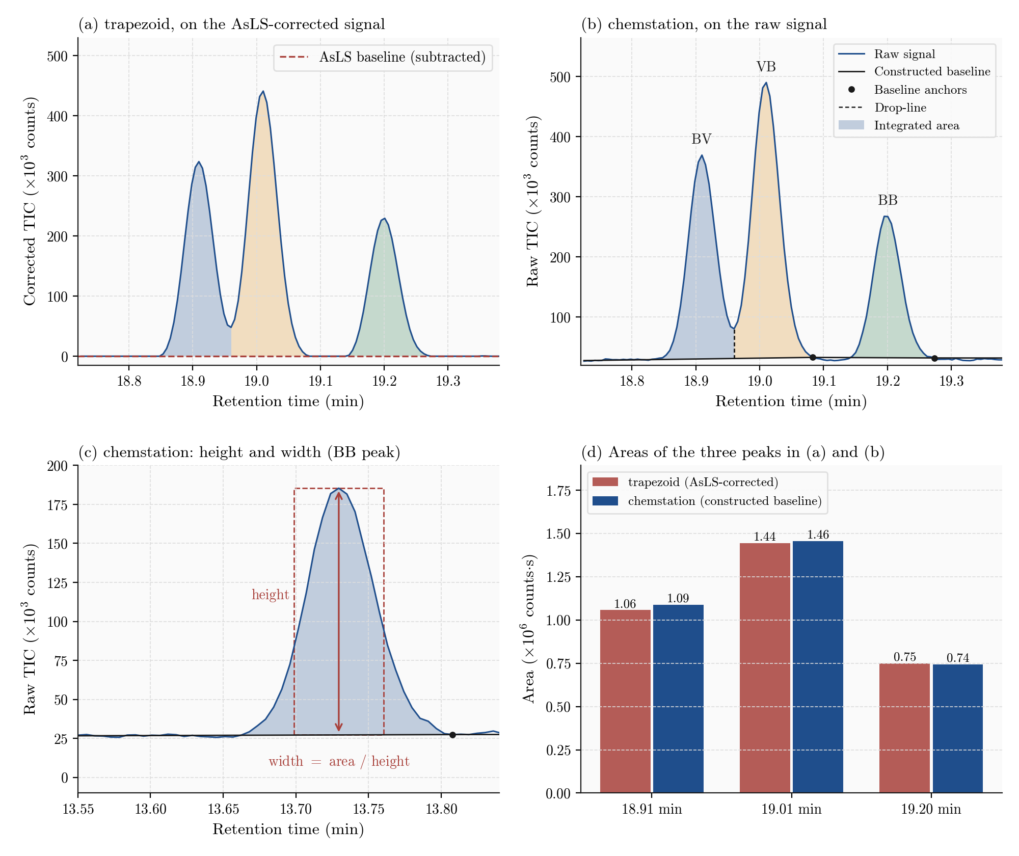
The same peaks integrated with the trapezoidal rule and with the vendor methodology — **Figure 5.** Integration on the synthetic triplet. (a) The trapezoidal rule on the AsLS-corrected signal, between the detected limits. (b) The vendor methodology on the raw signal: a constructed baseline through its anchor points, a drop-line between the first two peaks (codes `BV` and `VB`), and a third peak resolved to the baseline (`BB`). (c) The height and the equivalent-rectangle width reported for an isolated peak. (d) The resulting areas: the limits are identical, but the signal and the baseline differ, and so do the areas.

Units that are never conflated

An area is meaningless without its unit, and the units in play differ by orders of magnitude. The package reports every area in counts·min (the pivot), counts·s and counts·ms, the unit the vendor integrator carries internally. A fourth, clearly labelled reference-equivalent unit applies an empirical scale factor so computed areas can be placed next to the reference areas used for validation. Because that factor is not derived from the published methodology, it is kept out of the three physical units, calibrated once and reproducibly from the code, and never re-fitted per run, since a per-run fit would hide exactly the discrepancies validation exists to reveal.

From peaks to results

Identification and relative quantification

A reference table lists the compounds an analyst identified and their retention times. Each compound is matched to the nearest detected apex within a tolerance (±0.05 min, i.e. 3 s, by default). Compounds without a peak in tolerance are reported as unmatched rather than silently dropped.

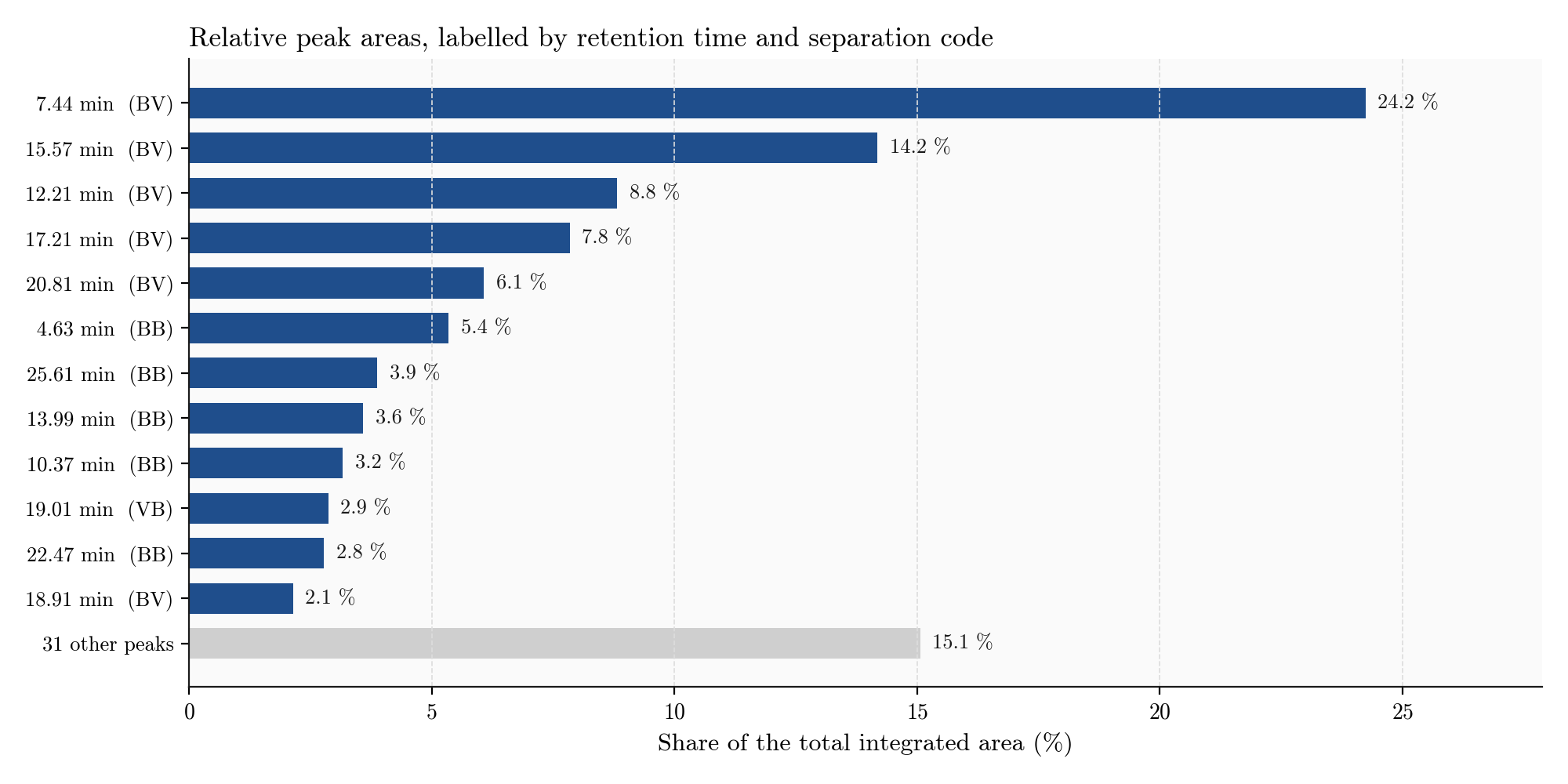
Without calibration standards, absolute concentrations cannot be recovered, so the quantitative readout is area normalisation: each peak’s area as a percentage of the total integrated area of its run. The result is a relative measure, computed within one run and in one unit, so the choice of unit cancels.

Relative areas of the largest synthetic peaks with their separation codes — **Figure 6.** Relative areas from the package's tidy peak table for the synthetic run: the twelve largest peaks, labelled by retention time and separation code, with the remaining peaks grouped. The shares sum to 100 % across the run.

Interactive reports and tidy exports

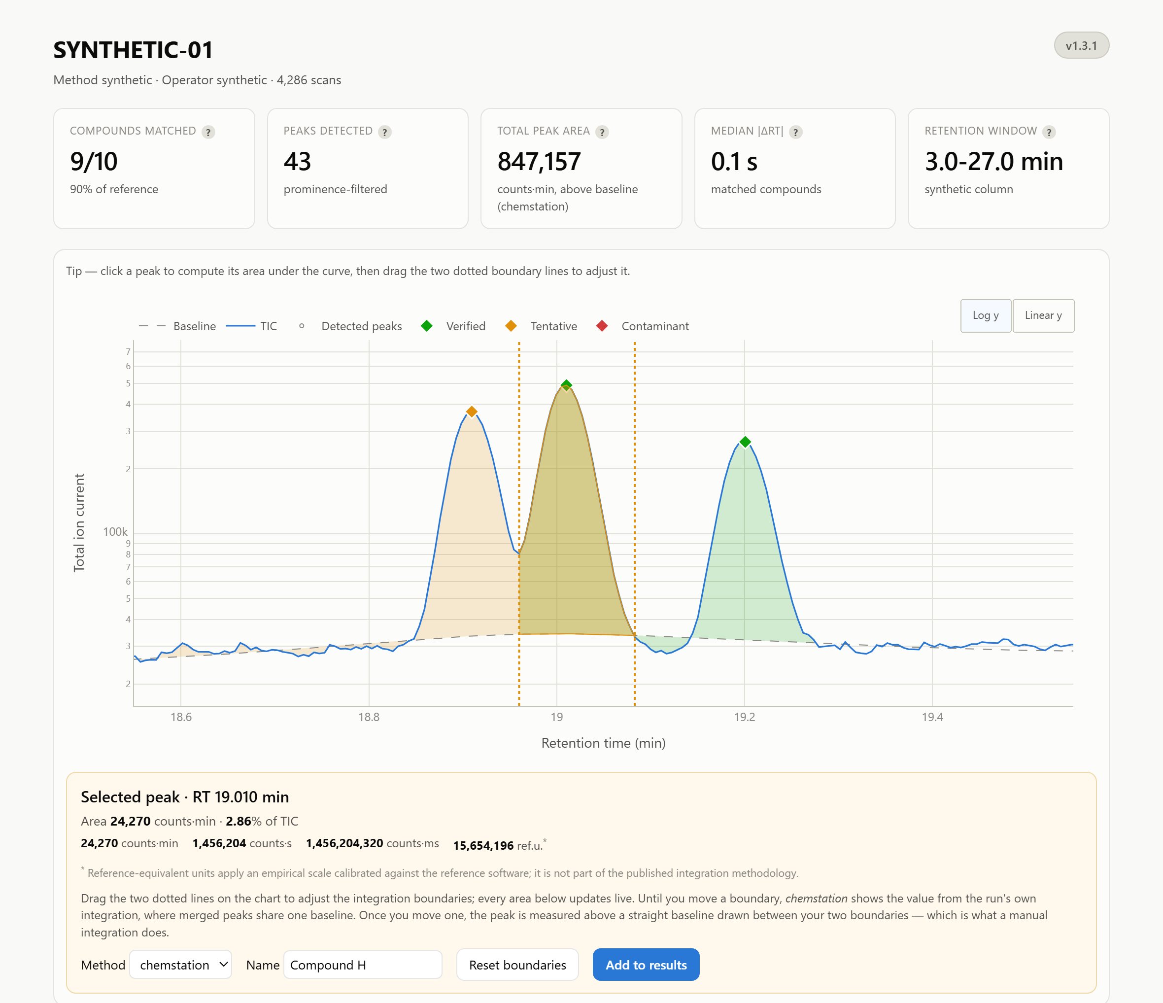
For inspection, the package renders a self-contained interactive HTML report per run (Plotly). The report shows the chromatogram with its baseline, every detected peak, matched compounds coloured by curation status, summary tiles and a results table. Clicking a peak shades and integrates it. Two boundary lines can then be dragged, and the area is recomputed live in every unit together with its share of the run. The integration method can be switched, and any peak, including one absent from the reference, can be named and added to the table. The table downloads as CSV, JSON or xlsx. The xlsx file is written in the browser without any dependency, so the report needs no server.

Screenshot of the interactive HTML report generated for the synthetic run — **Figure 7.** The interactive report generated by the package for the synthetic run, with fictitious reference compounds. The view is zoomed on the triplet, and the middle peak has been clicked: its limits appear as draggable dotted lines, and the panel gives its area in the four units and its share of the run.

For downstream analysis, exports are tidy tables, one row per compound with a run identifier, in CSV, JSON, Parquet or xlsx, per run and for a whole batch. Every column that carries a unit names it in its header, and every row records the integration method that produced it. A targeted command also integrates the peak nearest any retention time, whether or not it belongs to the reference.

Three interfaces, one library

All the logic lives in a typed Python library. A command-line tool exposes it as analyze, validate, report, export and integrate commands that accept single runs or whole directories. A desktop GUI (Tkinter) offers the same commands with native file pickers, contextual help on every parameter and processing on a background thread. It is also distributed as a standalone Windows executable that requires no Python installation. The interfaces are thin shells: the GUI’s integration menu, for instance, is populated from the integration registry, so it can never offer a method that is declared but not implemented.

Validation against manual results

Automating an analysis is only useful if the automated result can be trusted, so validation was built into the package as a first-class stage and run on real data (the data remain confidential, only aggregate results are reported here).

Identification. Over the runs that have both raw data and a manual identification table, detection places a peak within 3 s of the listed retention time for 209 of 225 compounds (93 %), with a median absolute error of about 0.1 s. The unmatched compounds are reported, not hidden. They are consistent with identifications made from mass spectra where no distinct peak is visible in the total-ion trace.

Areas. Computed areas were compared with a reference result set: 50 peaks integrated manually by an operator in four runs. A single overall difference would hide which stage disagrees, so the comparison is split into three tiers, each holding one stage fixed:

Tier	Integration limits	A discrepancy points to
Integration	the reference’s own limits	the integration method, baseline construction or unit
Bounds	detected limits compared with the reference’s	peak detection or boundary placement
End to end	detected limits	both combined

All 50 reference peaks are matched to a detected peak. Given the reference’s own limits, areas agree to a median of 3.5 % on the windows that start and end on the baseline. End to end, the median difference is 26.5 %, and the tiers show that it comes from boundary placement rather than from the integration method: the detector’s valley-to-valley windows are systematically wider than the narrow windows the operator drew by hand. The validation also flags two confounders instead of smoothing them away: every reference peak was integrated manually, and about half of the reference windows start or end part-way up a peak’s flank, where no automatic rule could reproduce them exactly.

Software architecture and reproducibility

The package is organised in strictly separated layers: configuration, data models, input/output, preprocessing, algorithms, interpretation, validation, presentation, orchestration and interfaces. Each algorithmic stage sits behind a strategy interface, so a new baseline or integration method can be added without touching the rest of the pipeline.

Reproducibility rests on three mechanisms. The processing parameters form a single, validated, frozen object whose short fingerprint (a hash of its content) identifies the exact configuration behind any output. Each signal carries a provenance tuple naming the transformations already applied. And a golden-file regression test freezes every detected apex and boundary on reference runs, so a change to detection cannot slip through unnoticed. When the default integration method changed, that test proved the detected peak set was unchanged.

The codebase is typed (mypy --strict), linted and formatted (ruff), covered by a test suite of just over 300 tests, run in continuous integration, and released with semantic versioning and a changelog. The scientific rationale, assumptions and literature references of every stage are documented alongside the code.

Limitations and next steps

One signal dimension. The pipeline works on the total-ion chromatogram, so compounds that co-elute but differ in mass are merged into one peak. Extracted-ion chromatograms would separate them.
Model-free peak splitting. Merged peaks are separated by drop-lines or valley baselines, not by fitting peak shapes. Heavily overlapping peaks would be apportioned more accurately by Gaussian or exponentially modified Gaussian deconvolution.
Detection sensitivity is a parameter. The prominence threshold decides how many minor features are retained, and deciding which peaks are worth reporting remains a separate choice.
Relative, not absolute, quantification. Area percentages assume comparable detector responses across compounds, which is only approximately true in GC-MS.
Identity from retention time only. Retention indices anchored on an n-alkane ladder and spectral library matching are the natural next steps towards instrument-independent identification.

Skills demonstrated

Signal processing and numerical methods: Savitzky–Golay filtering, penalised asymmetric least squares on sparse systems, robust noise estimation, prominence-based detection and numerical integration.
Analytical science: GC-MS data structures, chromatographic integration conventions (perpendicular drop, peak-valley ratio, separation codes), identification by retention time and area normalisation.
Reverse engineering and standards: a dependency-free parser for a binary vendor format, and an integration methodology reimplemented from its published documentation.
Validation and scientific rigour: tiered comparison against manual results that separates detection errors from integration errors, with confounders reported explicitly rather than tuned away.
Software engineering: a layered, typed, tested Python package with strategy interfaces, a method registry, versioned parameters, provenance tracking, golden-file regression tests and continuous integration.
Product delivery: a CLI, a desktop GUI packaged as a standalone executable, and self-contained interactive reports designed for users who do not program.

Conclusion

Integrating a peak is a few lines of code. Producing areas that a laboratory can trust, rerun and audit is an engineering project. This package turns a manual, operator-dependent workflow into a deterministic pipeline in which every decision (smoothing, baseline, detection threshold, limits, integration rule, unit) is explicit, parameterised and recorded. It reimplements the vendor’s integration methodology rather than inventing a new one, and it measures its own agreement with manual results before asking anyone to rely on it. Through a command line, a desktop application or a single HTML file, it puts that analysis in the hands of the people who produce the data.